Introduction

AI models and their training data are big. Training an AI model on only one GPU can become slow, and many models don't even fit on one single GPU. Many techniques exist to manage the memory and speed limitations of modern models. These techniques have unlocked many of the impressive advances in machine learning we see today. These training and inference techniques all depend on basic building blocks of collective communications called collective operations.

In this blog we will cover collective operations, how they are used to speed up training. We'll also discuss the unique way Burn implements collective operations in the 0.20.0 release, as well as how you can easily train your models on multiple devices and multiple nodes.

Data Parallel Training

Distributed data parallel training (DDP) is a basic example of distributed training. It consists of splitting the training data between multiple devices and training a copy of the model on each device, all while keeping the parameters in sync.

First, the training data is split between each device. Then, during each training step, each device does a forward and backward pass on its own batch of data. The resulting gradients are aggregated between each device. Each device then optimizes its model with the new gradients. At this point the models have the same optimized parameters.

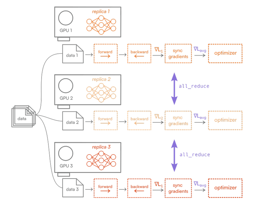
Figure 1: Data distributed training on three devices

This technique allows training time to be cut down significantly, as long as the gradient syncing is negligible. This technique still requires each device to store the entire model in memory, which is an issue tackled by other distributed training techniques.

It is clear that the key to this technique is the gradient syncing. The gradient syncing must be as efficient as possible as to not be a bottleneck in the pipeline.

Collective operations

The syncing of gradients in a data parallel training is a collecive operation called an all-reduce. An all-reduce is one of many primitive collective operations. Some others are:

• broadcast: one device sends a tensor to all others
• reduce: a tensor on each device is reduced to one tensor on one device
• reduce-scatter: a tensor on each device is reduced, each device ends up with a part of the resulting tensor

PyTorch and TensorFlow don't implement their own collective operations, instead they make use of communication libraries such as NCCL (for NVIDIA GPUs), MPI, or Gloo.

NCCL is the library used for NVIDIA GPUs. It abstracts collective operations using protocols like NVLink, PCIe, GPUDirect RDMA, and even TCP/IP. For all of NCCL's benefits, it is only useful for NVIDIA devices, which goes against Burn's core principles.

Moreover, Burn already has the tools for tensor communication between devices on the same machine with Tensor::to_device. We can take advantage of shared memory, or even backend specific protocols like NVLink for an Nvidia backend. Logically, GPU-to-GPU communication on the same machine should be done with to_device.

For these reasons, we decided to implement our own collective operations crate called burn-collective. For intra-node communication, we use Tensor::to_device, taking advantage of all the backend specific optimisations. For inter-node communication, we use TCP/IP. This two-step separation will show up later.

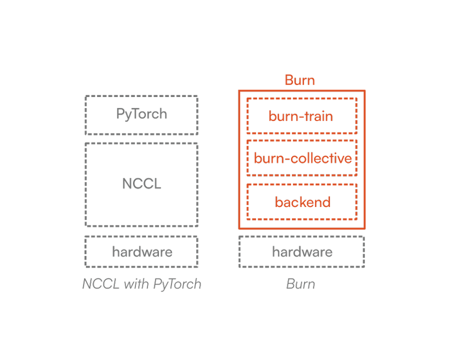
Figure 2: Pytorch and NCCL compared to Burn

How Burn implements collective operations

Burn currently only supports all-reduce. Reduce and broadcast are also supported, although only in single-node contexts.

How many processes?

We started with all-reduce, because it is the backbone to data distributed training.

With PyTorch, you usually assign a different process to each GPU. There are many reasons for this, but a big one is the Python's Global Interpreter Lock (GIL). The GIL only allows one thread to hold the Python interpreter at a time, which essentially prevents anything written in Python to actually be multi-threaded.

Thankfully, we're not using Python.

As said before, we can use to_device to take care of intra-node communication. We can assume the user will launch a thread for each GPU. So for one machine, we only need one process.

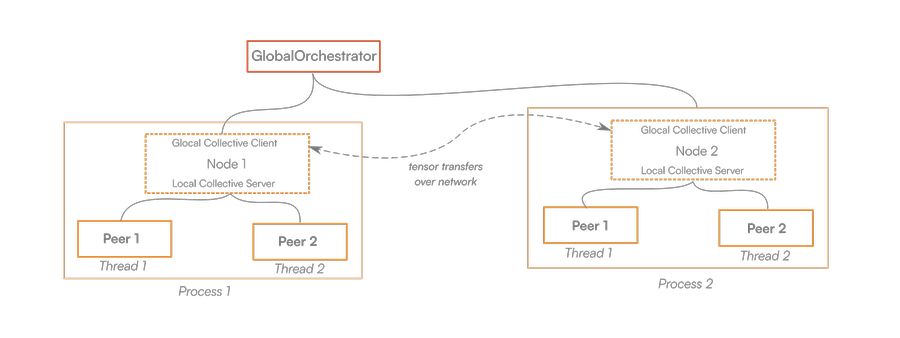Figure 3: Burn collective: an example structure with 4 peers and 2 nodes

Local and global

Since intra-node and inter-node communication are fundamentally different, we decided to split collective operations between a local (intra-node) and global (inter-node) level. Internally, the algorithms are implemented differently on the internal level and global levels.

This leads to a process-per-node structure.

It is worth noting that the local/global separation is an implementation detail, and it is only necessary to know when configuring the collective. From a user's perspective, all the other peers, whether on the same node or not, are just as accessible.

Walkthrough of an All-Reduce

Lets walk through the internals of a call to all_reduce

Each thread must first register, passing a CollectiveConfig that contains information about the number of peers on the same node, as well as the number of nodes in the collective. The call to register is blocking, so it syncs all the threads. When the node's LocalCollectiveServer has registered each peer on the node, the node will register on the global level if necessary.

Then, on the global level, the GlobalOrchestrator acts as a rendez-vous point for each node. After registering, the nodes have the addresses of every other node in the collective, and they can be as independent as possible. In the future, the GlobalOrchestrator could allow for a dynamic topology, keeping nodes updated on any changes.

Next, all peers in the collective call an all_reduce.

When all registered threads have called the opration, the LocalCollectiveServer starts the operation. In single node contexts, this is very simple, as the LocalCollectiveServer manages everything with Tensor::to_device for tensor transfers.

In a multi-node context, each node will already have the coordinates of other nodes, supplied upon registering. They communicate tensors with the burn_communications crate, specifically with the TensorDataService. This service allows for exposing and downloading Burn tensors over the network in a peer-to-peer manner. Currently we use WebSockets, but QUIC is a likely candidate for future use.

In multi-node contexts, nodes must synchronise at the end of the operation. This is true for all collective operations, but it becomes especially important for broadcast, where the broadcaster must wait for all receivers to receive the tensor.

Methods

Burn supports multiple strategies for all-reduce, configurable at both local and global levels.

Centralized

All peers send tensors to a root, which aggregates them and broadcasts the result back.

Tree

Peers are arranged in a b-tree and reduce in parallel, achieving $O(\log_b(N))$ time.

Ring

Peers form a ring, slicing tensors and passing them around. This maximizes bandwidth usage but is more sensitive to latency.

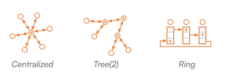
Figure 4: An overview of the three strategies

Local strategy and global strategy

Since the all-reduce is split on two levels, the local (intra-node) level and global (inter-node) level, we can use different local strategies for different nodes, and a different strategy on the global level. Below is a diagram that shows an example of a collective with 3 nodes, each using a different local strategy.

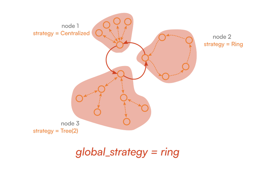
Local ring downfall

The Centralized and Tree strategies can be split into two operations: a reduce and a broadcast. A reduce operation aggregates all tensors onto one peer, and a broadcast distributes a tensor from one peer to all others.

The result from the global all-reduce needs to be broadcast to all other local peers. So, with Ring and Centralized we don't actually need to do a local all-reduce, we just need to do a reduce, followed by the global all-reduce, followed by the broadcast. It's like fitting the global all-reduce in the middle of the local all-reduce

So with Centralized and Tree in multi-node contexts we do:

Local reduce -> Global all-reduce -> Local broadcast

Due to the nature of the Ring algorithm, a ring-reduce can't be split between a reduce step and a broadcast step. This means if the Ring strategy is chosen locally, the steps will be as follows:

Local all-reduce -> Global all-reduce -> Local broadcast

This unnecessarily distributes the local all-reduce result to local peers, when anyway we will overwrite the tensor with the global all-reduce result. This may be less advantageous than other configurations. For this reason, it is recommended not to use Ring on the local level, only on the global level.

burn-communications

With the addition of burn-collective, it was necessary to build a solid base for network communication in burn. The burn-communications crate offers an abstraction of client-server logic, as well as a TensorDataService used for peer-to-peer tensor transfers. This allows developers to swap protocols with minimal effort.

DDP Training

Lets get back to a Data Parallel training. How can you take advantage of these fancy new collective operations?

Previously, to train on multiple devices, you had to use the LearnerBuilder::devices function:

let learner = LearnerBuilder::new(ARTIFACT_DIR)
    .devices(vec![gpu_1, gpu_2, gpu_3])
    // ...
    .build(model, config.optimizer.init(), 1e-4);

This has been replaced with LearnerBuilder::learning_strategy:

let collective = CollectiveConfig::default();

let learner = LearnerBuilder::new(ARTIFACT_DIR)
    .learning_strategy(burn::train::ddp(vec![gpu_1, gpu_2, gpu_3], collective))
    // ...
    .build(model, config.optimizer.init(), 1e-4);

The DDP learning strategy will launch a thread for each device, so in single-node environments this is a minimal change.

For multi-node environments, the user will need to launch the GlobalOrchestrator. After, they will need to launch the training on each node manually. Extra configuration is also required for the nodes to find each other.

let collective = CollectiveConfig::default()
    .with_global_address(Address::from_str("ws://example.com/orchestrator").unwrap())
    .with_num_nodes(3)
    .with_node_address(Address::from_str("ws://example.com/node_1").unwrap())
    .with_data_service_port(3000);

let learner = LearnerBuilder::new(ARTIFACT_DIR)
    .learning_strategy(burn::train::ddp(vec![gpu_1, gpu_2, gpu_3], collective))
    // ...
    .build(model, config.optimizer.init(), 1e-4);

Conclusion

With burn-collective and the new DDP learning strategy, training on multiple GPUs or even across multiple nodes is now straightforward in Burn. On a single machine, users only need to provide their devices—the framework handles threading and gradient synchronization automatically. Scaling to multiple nodes requires some extra configuration for the orchestrator and addresses, but the API stays consistent, and the communication layer abstracts away the complexity.

The key point is that you don’t need to learn NCCL, MPI, or low-level communication details. Burn provides a unified interface for collective operations that works across devices and nodes, while still letting you choose strategies that match your hardware. This makes it possible to start small and scale up without rewriting your training code.

If you’re already training models in Burn, upgrading to distributed data parallel training is just a few lines of code away.